Scatter plot of normalized categorical distributions

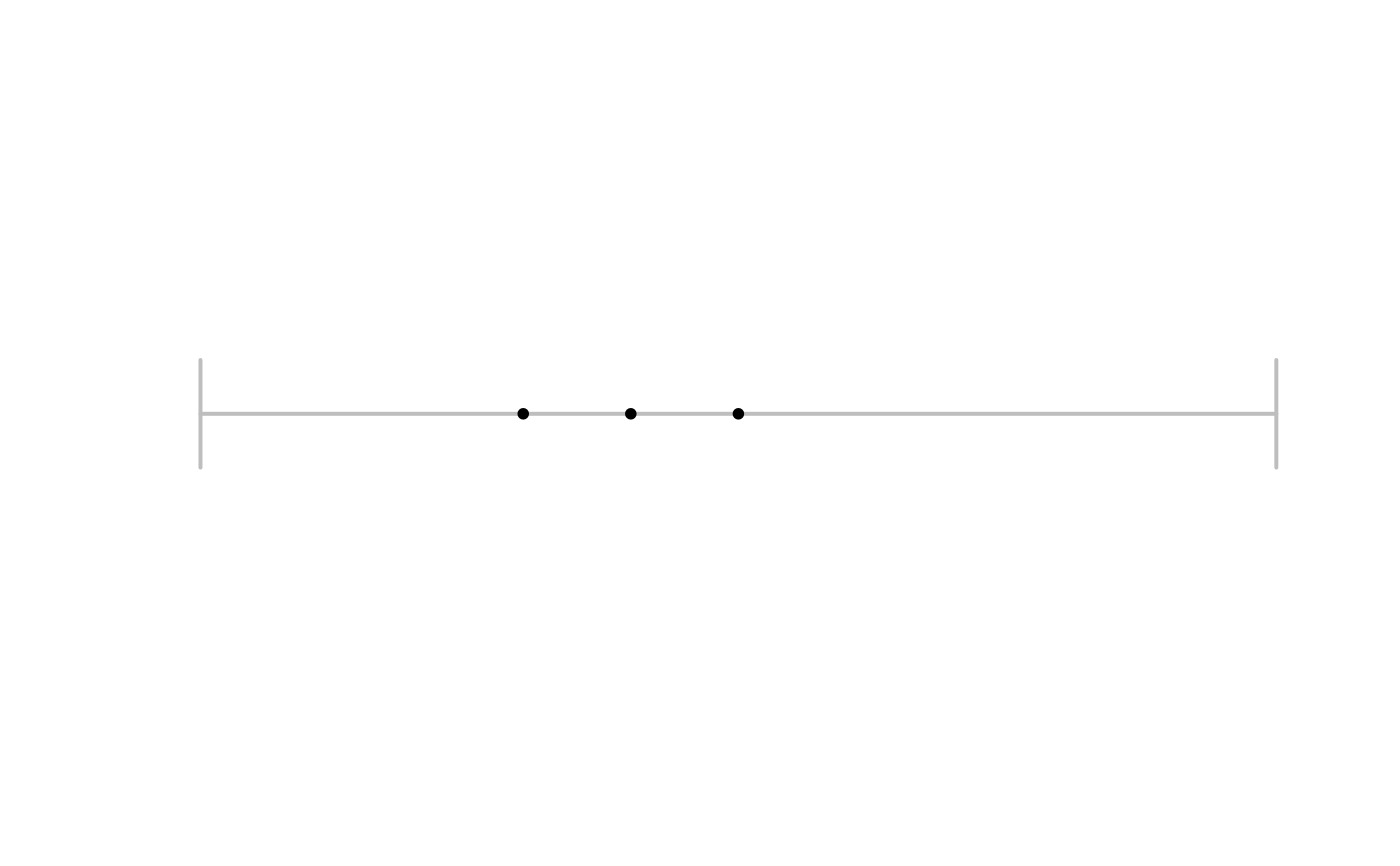
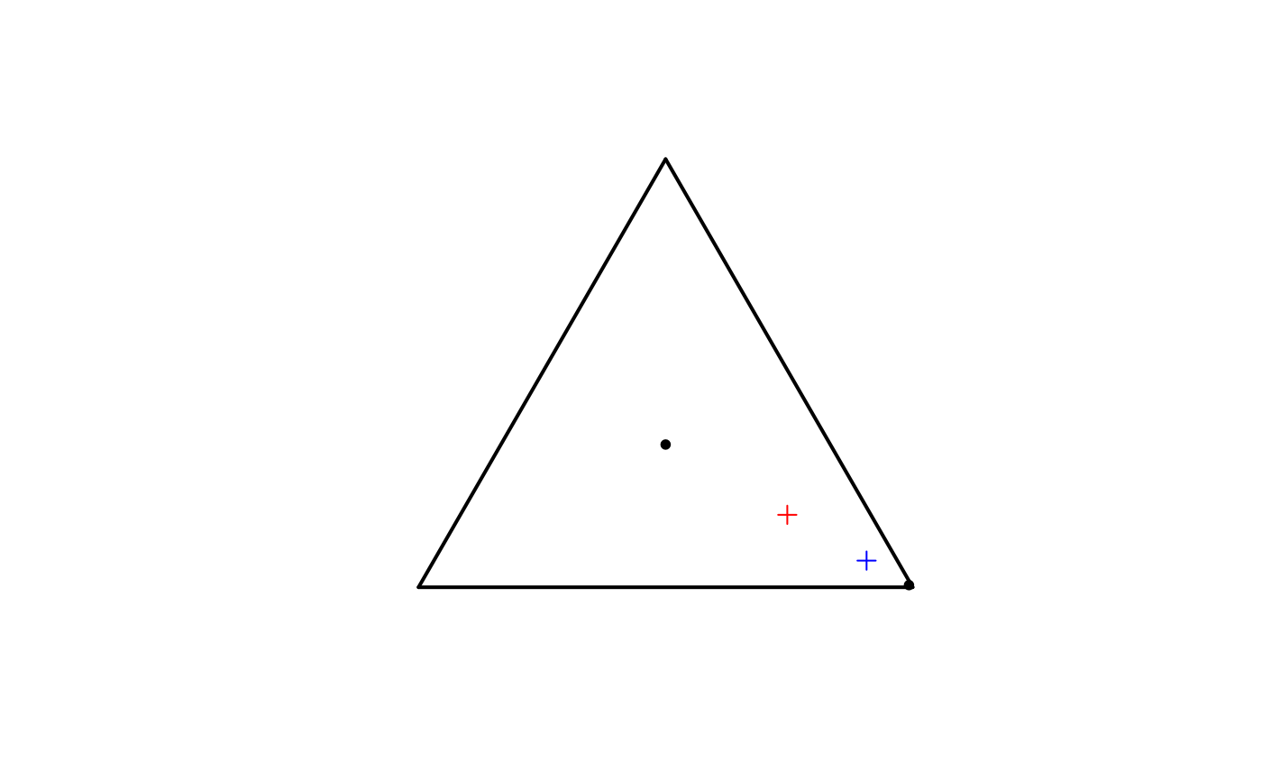
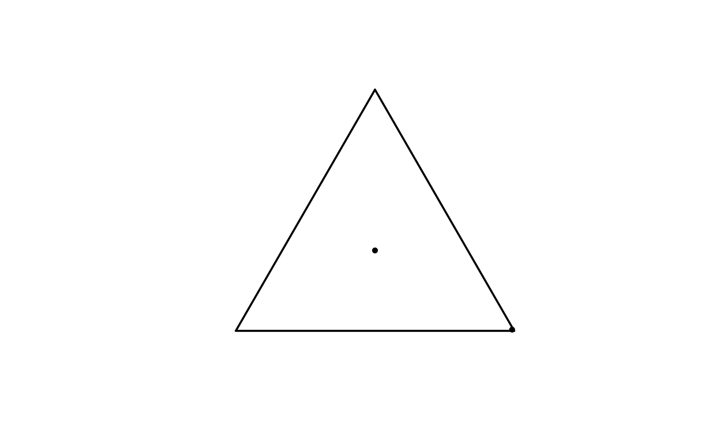
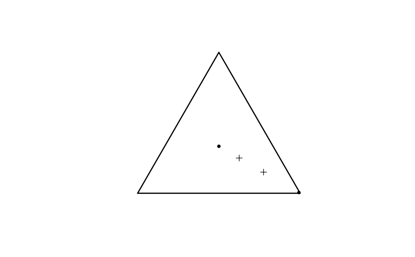
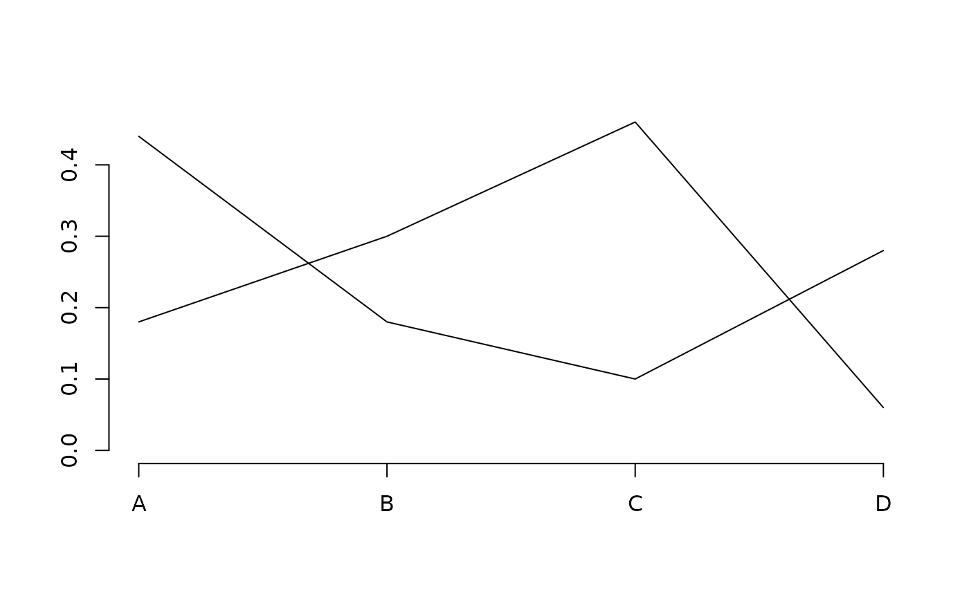
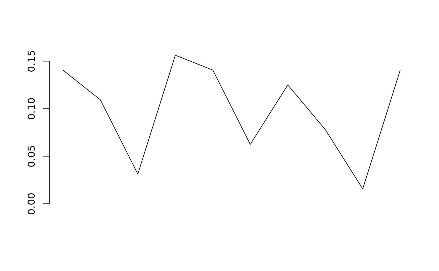
Methods plot() and points() for objects of classes igccatdistn and igcmatcatdistn. The type of the chart produced depends on the size of distributions to be drawn. More precisely, two-state distributions are drawn as points on a unit segment, three-state distributions are drawn as points in the equilateral triangle. Distributions with more than three states are drawn as polylines.

Usage

# S3 method for class 'igcmatcatdistn'
plot(x, y = NULL, add = FALSE, pch = 20, ...)

# S3 method for class 'igcmatcatdistn'
points(x, y = NULL, ...)

# S3 method for class 'igccatdistn'
plot(x, y = NULL, ...)

# S3 method for class 'igccatdistn'
points(x, y = NULL, ...)

Arguments

x

An object of class igcmatcatdistn, i.e., a matrice with positive entries and rows sum to 1.

y

NULL. Argument present only for compatibility with generic function plot.

add

Logical. Indicates whether the normalized categorical distributions should be drawn in a new chart (FALSE) or should be added to the active chart (TRUE).

pch

An integer value specifying the shape point

...

Further arguments to be passed to default methods for plot() and points(); see ?par for details.

Examples

# Two-state  categorical distributions plot
u <- c(0.5, 0.5)
p1 <- c(0.3, 0.7)
p2 <- c(0.4, 0.6)
x <- igcmatcatdistn(matrix(c(u, p1, p2),
                    nrow = 3, ncol = 2, byrow = TRUE))
plot(x)

# Three-state categorical distributions plot
u <- rep(1/3, 3)
prob <- c(0.99, 0.005, 0.005)
x <- matrix(c(u, prob),
            nrow = 2, ncol =3, byrow = TRUE)
x <- igcmatcatdistn(x)
plot(x)

# Many-state categorical distributions plot
set.seed(745)
var1 <- factor(sample(x = LETTERS[1:4], size = 50L,
                   replace = TRUE, prob = c(0.2, 0.3, 0.4, 0.1)),
            levels = LETTERS[1:4], ordered = TRUE)
p1 <- table(var1)
var2 <- factor(sample(x = LETTERS[1:4], size = 50L,
                   replace = TRUE, prob = c(0.4, 0.2, 0.1, 0.3)),
            levels = LETTERS[1:4], ordered = TRUE)
p2 <- table(var2)
p <- igcmatcatdistn(matrix(c(p1/sum(p1), p2/sum(p2)),
                           nrow = 2, ncol = 4, byrow = TRUE))
plot(p)
axis(side = 1, at = 1:4, labels = LETTERS[1:4])


u <- rep(1/3, 3)
prob <- c(0.99, 0.005, 0.005)
x <- matrix(c(u, prob),
            nrow = 2, ncol =3, byrow = TRUE)
x <- igcmatcatdistn(x)
plot(x)
y <- matrix(c(0.7, 0.15, 0.15,
              0.5, 0.25, 0.25),
              nrow = 2, ncol = 3, byrow = TRUE)
y <- igcmatcatdistn(y)
points(y, pch = 3)

p <- sample(1:10, size = 10L, replace = TRUE)
p <- igccatdistn(p/sum(p))
plot(p)

u <- rep(1/3, 3)
prob <- c(0.99, 0.005, 0.005)
x <- matrix(c(u, prob),
            nrow = 2, ncol =3, byrow = TRUE)
x <- igcmatcatdistn(x)
plot(x)
acent <- arithcent(p = x)
acent <- igccatdistn(acent)
gcent <- geomcent(p = x)
gcent <- igccatdistn(gcent/sum(gcent))
points(x = acent, pch = 3, col = "red")
points(x = gcent, pch = 3, col = "blue")